Mapping Quantum States: Exploring the Geometry of Hilbert Space

Date: 26 March 2026

In our previous blog, we explored the mathematical backbone of the quantum world: Vector Spaces. We learned that a Hilbert Space is essentially a “complete” vector space equipped with an inner product, a ruler to measure the similarity between quantum states.

But once you step inside this space, how do you find your way around? How do we turn an abstract quantum state into a clear map of information? Today, we dive deeper into the geometry of Hilbert Space and the secret code scientists use to talk to it.

The Perfect Room: Completeness and Dimension

As we discussed previously, a Hilbert Space is a complete space.

In simple terms:

Finite Dimensions: If your quantum system is small (like a single photon’s polarization), it is naturally “closed” and complete.
Infinite Dimensions: In more complex systems (like light waves), we assume completeness so that our mathematical “approximations” always land on a real, physical result.

While the theory is deep, for most optical quantum communications, thinking of it as a well-behaved Inner-Product Vector Space is often enough to get the job done!

Orthogonality: Staying Out of Each Other’s Way

In a Hilbert Space, the most important relationship between two vectors (or quantum states) is Orthogonality.

Two quantum states vectors $|x\rangle$ and $|y\rangle$ are orthogonal if their inner product is zero:

$\langle x,y \rangle =0$

In our previous post, we mentioned the inner product determines similarity. If the result is zero, it means the states are perfectly independent like two radio stations on completely different frequencies that never interfere.

Building the Map: Orthonormal Bases

To describe any point in space, you need a Basis (like North, South, East, and West). In Quantum Mechanics, we prefer an Orthonormal Basis.

This means:

Every direction is at a 90-degree angle to the others (Orthogonal).
Every direction has a “length” of exactly 1 (Normal).

We use the Kronecker Symbol $\delta_{ij}$ to represent this perfectly organized grid:

$\delta_{ij} = 1$ if you are looking at the same direction ( $i=j$ ).

$\delta_{ij} = 0$ if you are looking at different directions ( $i \neq j$ ).

Coordinate Systems and Fourier Expansion

Once we have our “Quantum Map” (the Basis), any state $|x\rangle$ can be written as a unique combination of those directions. This is called Fourier Expansion.

Think of it like GPS coordinates. Instead of saying “the particle is somewhere over there,” we say:

The particle is $a_1$ units of Direction A + $a_2$ units of Direction B.

The coordinates $a_i$ are found simply by taking the inner product:

$a_i =\langle b_i | x \rangle$

The Language of the Pros: Dirac’s “Bra-ket” Notation

To make these calculations easier, we use Dirac’s Notation. It splits the word “Bracket” into two parts to describe the vectors we introduced in the last blog:

The Ket $| x \rangle$ : A column vector (the quantum state itself).

The Bra $\langle x |$ : A row vector (the “mirror” of the state).

The Inner Product $\langle x | y \rangle$ : The “Bracket” that measures how much two states overlap.

Concept	Standard Notation	Dirac Notation
Vector	$x$	$x$
Orthogonality	$\langle x , y \rangle$	$\langle x \| y \rangle$
Length (Norm)	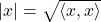$\|x\|= \sqrt{\langle x , x \rangle}$	$\|x\|= \sqrt{\langle x \| x \rangle}$

By establishing a coordinate system in a Hilbert Space, we can translate physical quantum particles into digital-like coordinates in $\mathbb{C}^n$ .

This allows us to process, transmit, and secure information using the laws of physics.

Whether we are dealing with periodic signals or discrete pulses, the Hilbert Space ensures that our “quantum map” is always accurate, complete, and ready for communication.

Mapping Quantum States: Exploring the Geometry of Hilbert Space

Published by Quantum Communications on March 26, 2026March 26, 2026